Quickstart
In this section, we demonstrate how to use TMMax to compute and visualize the reflection and transmission spectra of a multilayer thin-film stack. This walkthrough aims to guide you through each step of the process: from defining the material structure and simulation parameters to extracting the optical response under different polarizations.
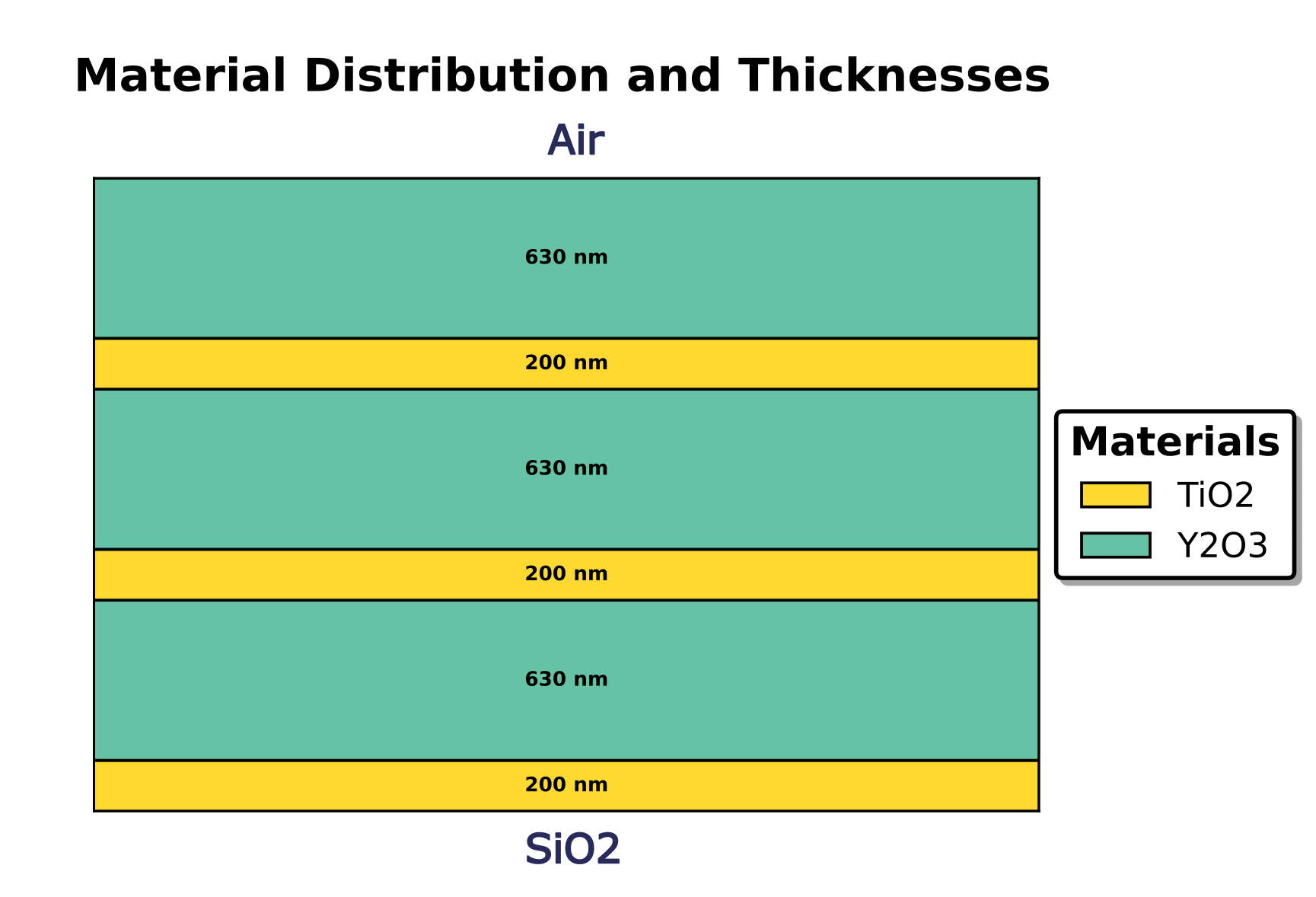
Here, we consider a coherent multilayer system composed of alternating high- and low-refractive-index layers, arranged as:
This example serves as an accessible introduction to TMMax and illustrates the workflow from simulation setup to data visualization.
Step 1: Import the Required Libraries
The first step is to import the numerical and simulation libraries. We rely on jax.numpy for defining arrays (angles of incidence, wavelengths, and thicknesses) because TMMax is built to leverage JAX’s performance and automatic differentiation capabilities. The core TMMax simulation engine is accessed through the tmm function:
import jax.numpy as jnp
from tmmax.tmm import tmm
jax.numpy: Provides the same interface as NumPy but supports JAX’s accelerated computations on CPU, GPU, or TPU.tmmThe transfer matrix method solver from TMMax, which computes reflection (R) and transmission (T) spectra for multilayer thin-film stacks.
Step 2: Define the Multilayer Structure and Simulation Parameters
Next, we describe the multilayer structure and specify the simulation parameters. The materials are defined as a Python list, and the thickness values are assigned using a JAX array (jnp.array). We also define the wavelength range and the angular range of incidence:
material_list = ["Air", "Y2O3", "TiO2", "Y2O3", "TiO2", "Y2O3", "TiO2", "SiO2"]
thickness_list = jnp.array([630e-9, 200e-9, 630e-9, 200e-9, 630e-9, 200e-9])
wavelength_arr = jnp.linspace(500e-9, 700e-9, 1000)
angle_of_incidences = jnp.linspace(0, (70*jnp.pi/180), 1000)
material_list: Defines the sequence of layers in the multilayer stack. The first layer is air (ambient), followed by alternating layers of Y₂O₃ (yttrium oxide) and TiO₂ (titanium dioxide), and finally SiO₂ (substrate).thickness_list: Specifies the physical thickness of each thin film in the stack, in meters. For example, Y₂O₃ layers are 630 nm thick, while TiO₂ layers are 200 nm thick.wavelength_arr: The spectral range for simulation, spanning from 500 nm to 700 nm with 1000 sampling points.angle_of_incidences: The incidence angle range, sweeping from 0° (normal incidence) up to 70°, also sampled at 1000 points.
Step 3: Choose Polarization and Run the Simulation
The reflection and transmission depend on the polarization of light. TMMax allows us to compute spectra for s-polarized (perpendicular) and p-polarized (parallel) light. We first calculate the spectra for s-polarized light:
polarization = 's'

R_s, T_s = tmm(material_list = material_list,
               thickness_list = thickness_list,
               wavelength_arr = wavelength_arr,
               angle_of_incidences = angle_of_incidences,
               polarization = polarization)
polarization = 's': Specifies s-polarization.R_s,T_s: Arrays containing the reflection and transmission coefficients, respectively, as functions of wavelength and angle of incidence.
We can repeat the calculation for p-polarized light by changing the polarization parameter:
polarization = 'p'

R_p, T_p = tmm(material_list = material_list,
               thickness_list = thickness_list,
               wavelength_arr = wavelength_arr,
               angle_of_incidences = angle_of_incidences,
               polarization = polarization)
Step 4: Visualize Reflection and Transmission
Finally, we visualize the computed reflection and transmission spectra. The plots provide an intuitive understanding of how the multilayer stack interacts with incoming light. Reflection and transmission spectra are often complementary, showing how much light is reflected versus transmitted at different wavelengths and angles.
Reflection Spectrum:
import matplotlib.pyplot as plt
from mpl_toolkits.axes_grid1 import ImageGrid

# Set up figure and image grid
fig = plt.figure(figsize=(10, 5))

grid = ImageGrid(fig, 111,
                nrows_ncols=(1,2),
                axes_pad=0.65,
                share_all=True,
                cbar_location="right",
                cbar_mode="single",
                cbar_size="5%",
                cbar_pad=0.25,
                )

# Add data to image grid
i = 0
for ax in grid:
    if i == 0:
        im = ax.imshow(result_s[0]*100, cmap='Spectral', aspect=200/70,extent = [500, 700, 0, 70])
        ax.set_title("s-polarization")
    if i ==1:
        im = ax.imshow(result_p[0]*100, cmap='Spectral', aspect=200/70,extent = [500, 700, 0, 70])
        ax.set_title("p-polarization")
    ax.set_xlabel("Wavelength (nm)")
    ax.set_ylabel("Incident angle ($^o$)")
    i += 1

# Colorbar
ax.cax.colorbar(im, label='Reflectance (%)')
plt.show()
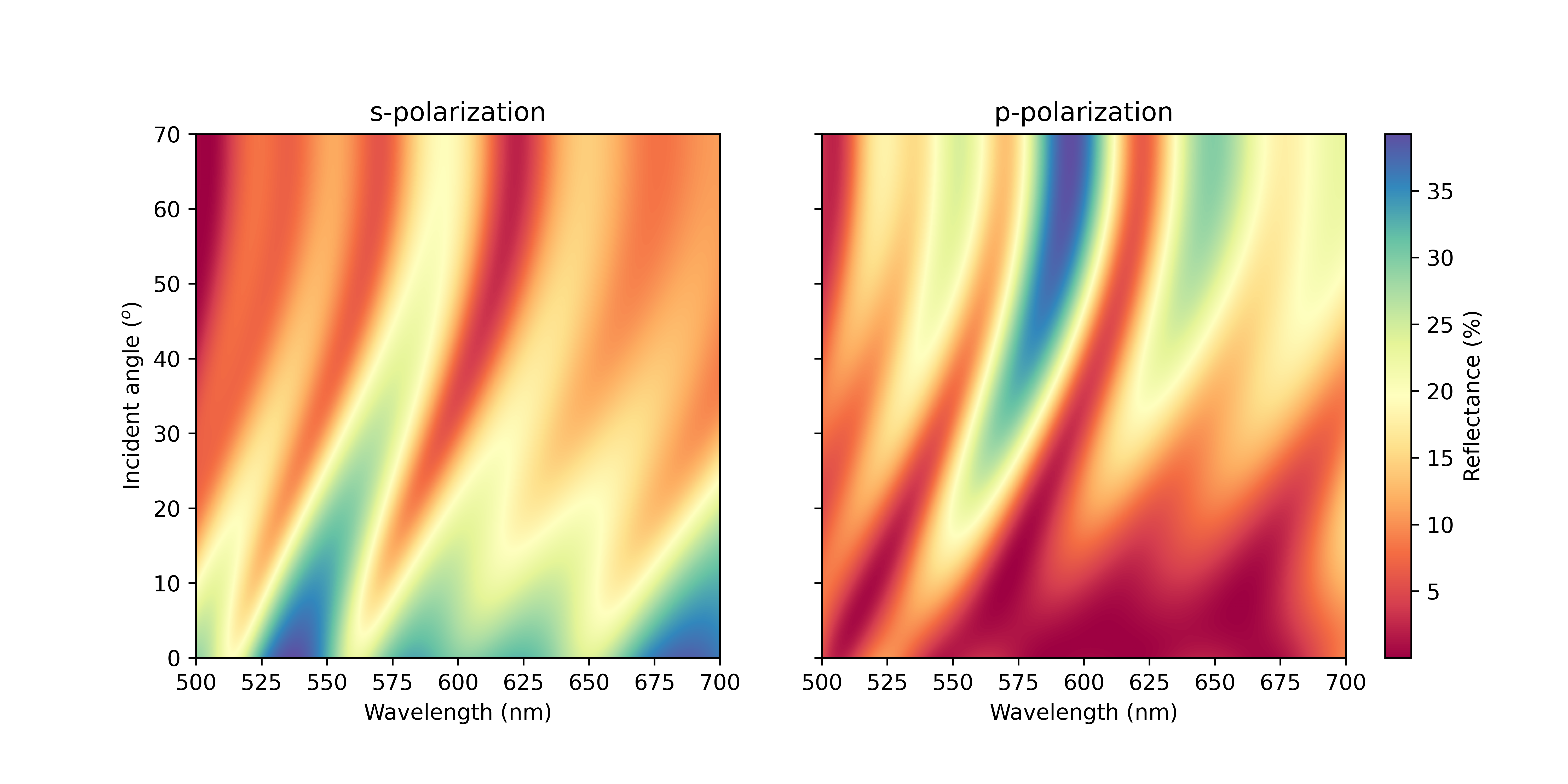
Reflection spectrum of the multilayer stack for s-polarized light. The figure shows reflection intensity as a function of both wavelength and angle of incidence.
Transmission Spectrum:
import matplotlib.pyplot as plt
from mpl_toolkits.axes_grid1 import ImageGrid

# Set up figure and image grid
fig = plt.figure(figsize=(10, 5))

grid = ImageGrid(fig, 111,
                nrows_ncols=(1,2),
                axes_pad=0.65,
                share_all=True,
                cbar_location="right",
                cbar_mode="single",
                cbar_size="5%",
                cbar_pad=0.25,
                )

# Add data to image grid
i = 0
for ax in grid:
    if i == 0:
        im = ax.imshow(result_s[1]*100, cmap='Spectral', aspect=200/70,extent = [500, 700, 0, 70])
        ax.set_title("s-polarization")
    if i ==1:
        im = ax.imshow(result_p[1]*100, cmap='Spectral', aspect=200/70,extent = [500, 700, 0, 70])
        ax.set_title("p-polarization")
    ax.set_xlabel("Wavelength (nm)")
    ax.set_ylabel("Incident angle ($^o$)")
    i += 1

# Colorbar
ax.cax.colorbar(im, label='Transmittance (%)')
plt.show()
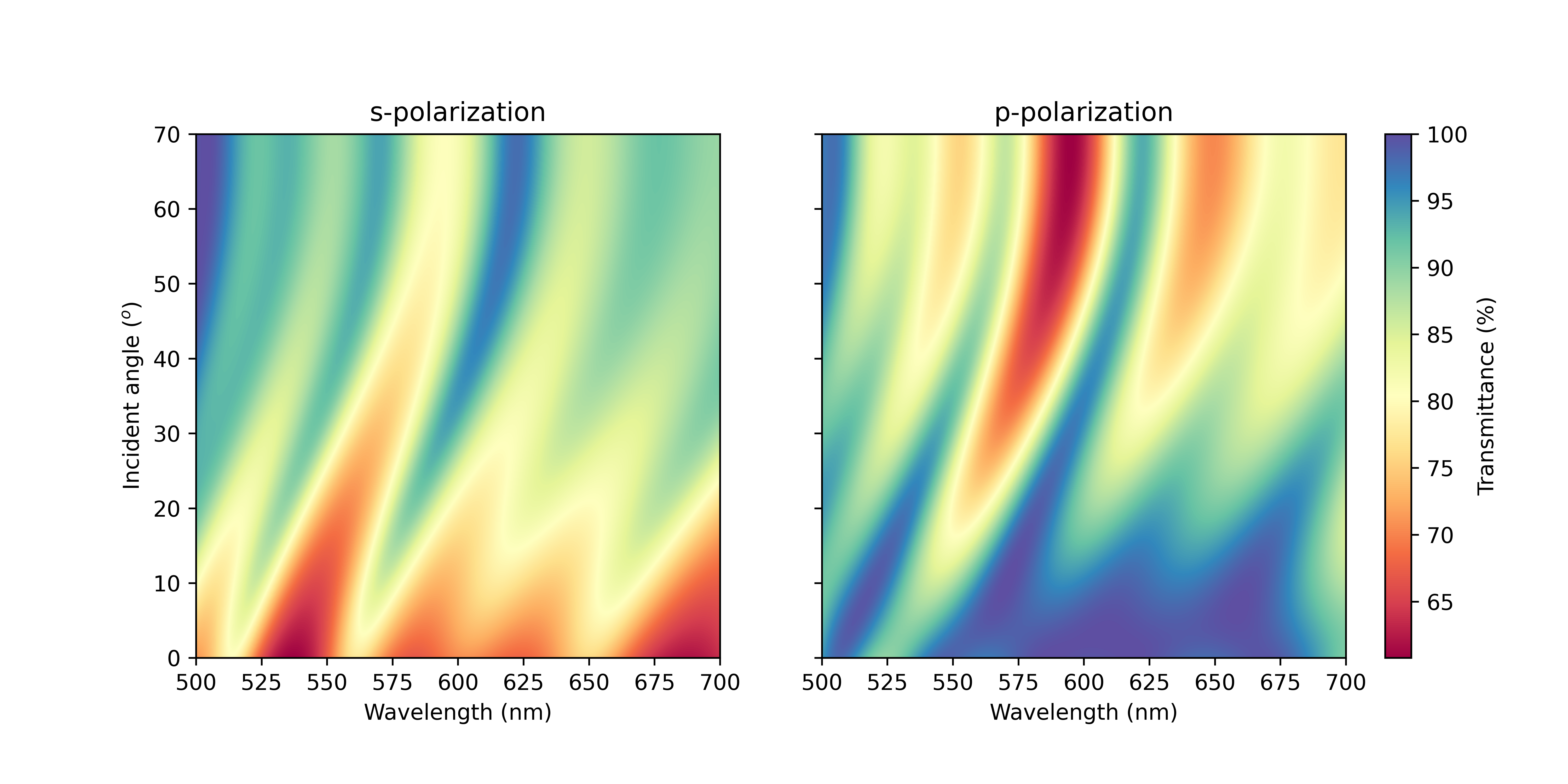
Transmission spectrum of the multilayer stack for s-polarized light. The figure shows transmission intensity as a function of both wavelength and angle of incidence.
The plotted figures for reflection and transmission provide valuable insights into the system’s optical performance. In practice, such simulations form the foundation of thin-film engineering, where optimized stacks are designed for applications like anti-reflective coatings, photonic crystals, or high-reflectivity dielectric mirrors. TMMax makes this process accessible and efficient, combining numerical accuracy with computational speed.