Python Implementation
In this section, we implement the TMM algorithm using the tmmax library, which is designed for high-performance multilayer simulations with vectorized operations using the jax library.
[ ]:
!pip install tmmax
Requirement already satisfied: tmmax in /usr/local/lib/python3.10/dist-packages (0.1.0)
Visualizing Refractive Index and Extinction Coefficient Data
[ ]:
import jax.numpy as jnp
from tmmax.data import visualize_material_properties
import matplotlib.pyplot as plt
### Refractive Index and Extinction Coefficient as a Function of Wavelength
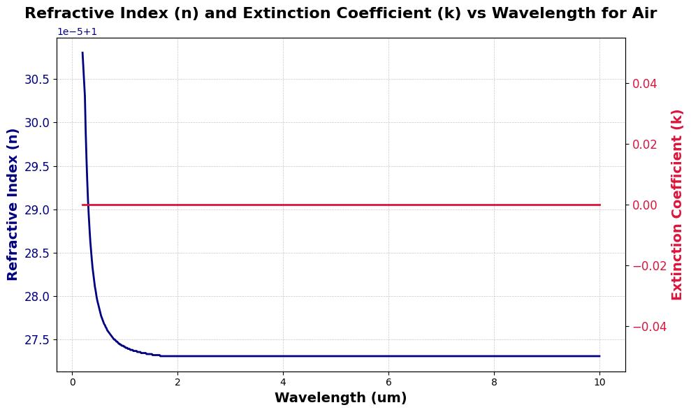
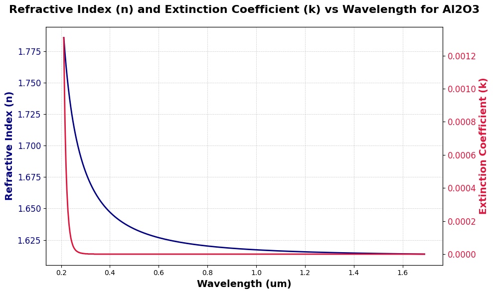
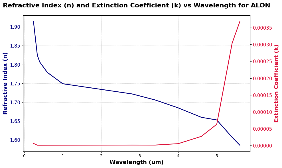
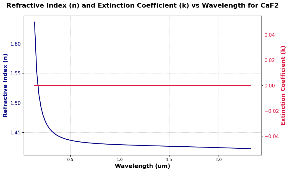
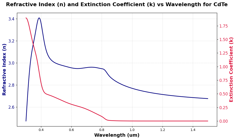
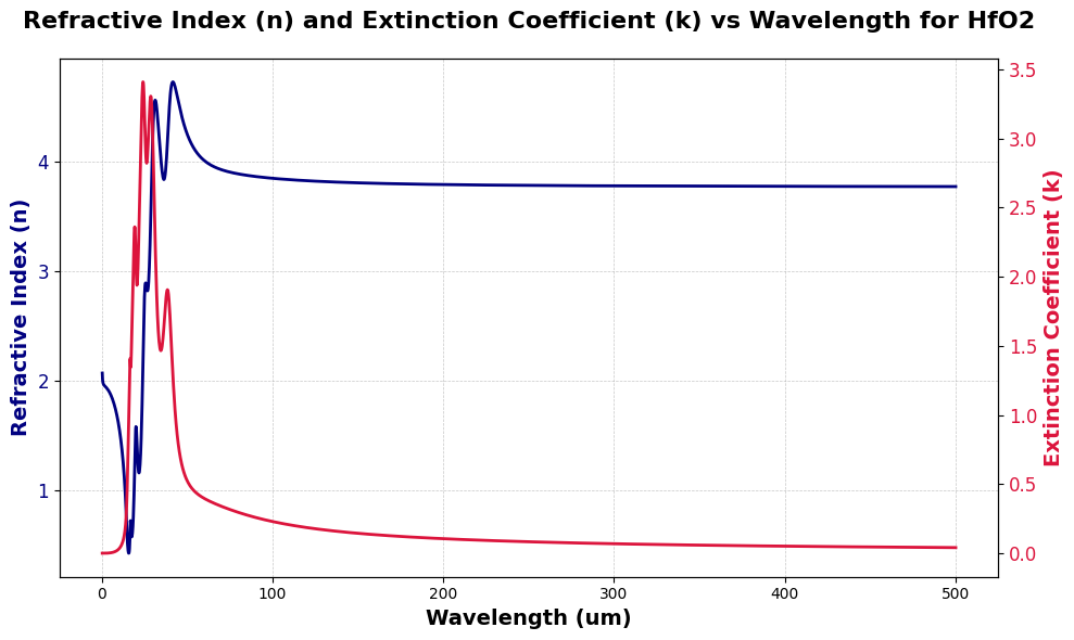
As of May 6, 2025, the visualizations of all materials available in the tmmax database are provided below. We can visualize the refractive index (n) and extinction coefficient (k) as a function of wavelength. This uses data from the internal nk database and plots it with dual y-axes (n on left, k on right)
[ ]:
visualize_material_properties(material_name = "Air")
[ ]:
visualize_material_properties(material_name = "Al2O3")
[ ]:
visualize_material_properties(material_name = "ALON")
[ ]:
visualize_material_properties(material_name = "CaF2")
[ ]:
visualize_material_properties(material_name = "CdS")

[ ]:
visualize_material_properties(material_name = "CdTe")
[ ]:
visualize_material_properties(material_name = "CeF3")

[ ]:
visualize_material_properties(material_name = "Ge")

[ ]:
visualize_material_properties(material_name = "HfO2")
[ ]:
visualize_material_properties(material_name = "SiO2")

### Logarithmic Scale Axis
Either axis can be converted to a logarithmic scale using the logX and logY flags.
[ ]:
visualize_material_properties(material_name = "SiO2", logX = True, logY = False)

[ ]:
visualize_material_properties(material_name = "SiO2", logX = False, logY = True)

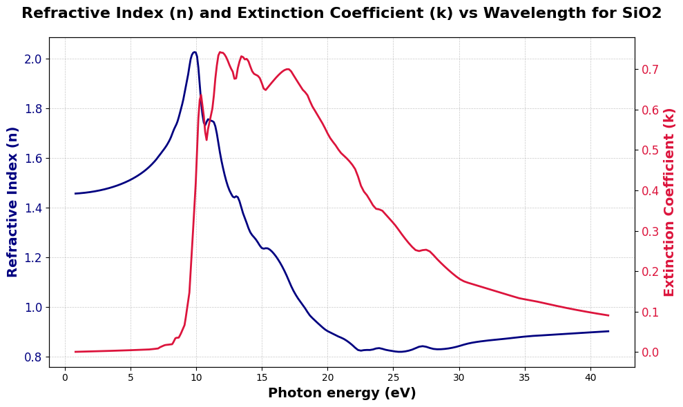
### Refractive Index and Extinction Coefficient as a Function of Photon Energy
You can also display the x-axis in terms of photon energy instead of wavelength. To do this, simply enable the eV flag.
[ ]:
visualize_material_properties(material_name = "SiO2", logX = False, logY = False, eV = True)
### Saving Plot
If you want to save the plot of this data, set savefig = True and then provide the folder name as a string to save_path. Please do not enter the full path.
[ ]:
visualize_material_properties(material_name = "SiO2", logX = False, logY = False, eV = True, savefig = True, save_path = "material_info/SiO2_data")
Figure saved successfully at: material_info/SiO2_data/SiO2_nk_plot.png

Adding Refractive Index and Extinction Coefficient Data to Material Database
Importing Libraries
Importing visualize_material_properties function from tmmax.data is sufficient for data visualizations.
[ ]:
import jax.numpy as jnp
from jax import jit
from tmmax.data import add_material_to_nk_database
Creating Dummy n, k Data Generator Function
Here, I created a function that generates n and k data for a dummy material. In your case, this is not necessary—you can directly use your own n and k data.
[ ]:
@jit
def dummy_material_n_k(wavelength_um):
    """
    Calculate refractive index and extinction coefficient for dummy material

    Args:
        wavelength_um: Wavelength in micrometers (1.5-1.6 um range)

    Returns:
        n: Refractive index
        k: Extinction coefficient
    """
    # Create a fake wavelength-dependent refractive index with some features
    n_base = 3.2
    n_peak = 0.15 * jnp.exp(-((wavelength_um - 1.55) / 0.02)**2)
    n = n_base + n_peak

    # Create a fake wavelength-dependent extinction coefficient
    k_base = 0.001
    k_peak = 0.0005 * jnp.exp(-((wavelength_um - 1.53) / 0.03)**2)
    k = k_base + k_peak

    return n, k
Creating dummy_n and dummy_k data arrays.
[ ]:
dummy_wavelengths = jnp.linspace(1.5, 1.6, 100)
dummy_n, dummy_k = dummy_material_n_k(dummy_wavelengths)
Adding Materials to the Database
The following line adds a new material named 'dummy_material' to the internal n-k database. It takes four arguments:
wavelength_arr: an array of wavelength values,refractive_index_arr: an array representing the real part of the refractive index (n),extinction_coeff_arr: an array representing the imaginary part (k),material_name: the name of the material to be added.
In this example, dummy data (dummy_wavelengths, dummy_n, and dummy_k) is used to simulate a material entry. In practice, you can replace these arrays with your actual n and k data.
[ ]:
add_material_to_nk_database(wavelength_arr = dummy_wavelengths,
                            refractive_index_arr = dummy_n,
                            extinction_coeff_arr = dummy_k,
                            material_name='dummy_material')
'dummy_material.csv' recreated successfully.
Plotting the Material Data
You can directly plot the materials you’ve added to the database using visualize_material_properties.
[ ]:
visualize_material_properties(material_name = "dummy_material")

Reflectance Performance of the W-coat on a Glass Substrate
Introduction
We will use the Transfer Matrix Method (TMM) to analyze the reflection behavior of this multilayer thin film. The W-coat consists of two layers made from Magnesium Fluoride (MgF₂) and Yttrium Oxide (Y₂O₃). These layers are stacked on a glass substrate (Silicon Dioxide, SiO₂), and the incident medium is air.
In this example, the calculation is done for two polarizations:
s-polarization: Electric field perpendicular to the plane of incidence.
p-polarization: Electric field parallel to the plane of incidence.
We will calculate the reflectance as a function of wavelength and angle of incidence for each polarization.
Materials and Layer Thickness
We are considering the following material stack:
Air as the incident medium.
MgF₂ (Magnesium Fluoride) with a thickness of 93 nm.
Y₂O₃ (Yttrium Oxide) with a thickness of 63 nm.
SiO₂ (Silicon Dioxide) as the substrate.
These materials are well-suited for anti-reflection coatings and optical filters due to their refractive indices.
[ ]:
from tmmax.tmm import tmm

# Define the materials and their thicknesses
material_list =  ["Air", "MgF2", "Y2O3", "SiO2"]
thickness_list = jnp.array([93e-9, 63e-9])

# Define the wavelength range (500 nm to 700 nm) and angles of incidence (0° to 70°)
wavelength_arr = jnp.linspace(500e-9, 700e-9, 1000)
angle_of_incidences = jnp.linspace(0, (70*jnp.pi/180), 1000)

# Calculate reflectance for s-polarization
result_s = tmm(material_list=material_list, thickness_list=thickness_list,
             wavelength_arr=wavelength_arr, angle_of_incidences=angle_of_incidences,
             polarization="s")

# Calculate reflectance for p-polarization
result_p = tmm(material_list=material_list, thickness_list=thickness_list,
             wavelength_arr=wavelength_arr, angle_of_incidences=angle_of_incidences,
             polarization="p")
Visualization of Results
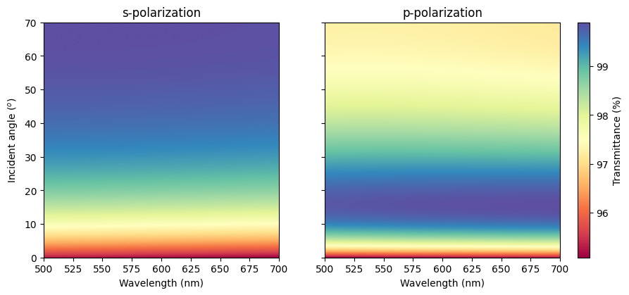
We will now visualize the reflectance, transmittance and absorbance for both s-polarization and p-polarization as a function of wavelength and angle of incidence. The color map will represent the reflectance percentage.
Reflectance Results
[ ]:
import matplotlib.pyplot as plt
from mpl_toolkits.axes_grid1 import ImageGrid

# Set up figure and image grid
fig = plt.figure(figsize=(10, 5))

grid = ImageGrid(fig, 111,
                 nrows_ncols=(1,2),
                 axes_pad=0.65,
                 share_all=True,
                 cbar_location="right",
                 cbar_mode="single",
                 cbar_size="5%",
                 cbar_pad=0.25,
                 )

# Add data to image grid
i = 0
for ax in grid:
    if i == 0:
        im = ax.imshow(result_s[0]*100, cmap='Spectral', aspect=200/70,extent = [500, 700, 0, 70])
        ax.set_title("s-polarization")
    if i ==1:
        im = ax.imshow(result_p[0]*100, cmap='Spectral', aspect=200/70,extent = [500, 700, 0, 70])
        ax.set_title("p-polarization")
    ax.set_xlabel("Wavelength (nm)")
    ax.set_ylabel("Incident angle ($^o$)")
    i += 1

# Colorbar
ax.cax.colorbar(im, label='Reflectance (%)')

plt.savefig("w_coat_reflectance_s_p.png", dpi=600)
plt.show()

Transmittance Results
[ ]:
# Set up figure and image grid
fig = plt.figure(figsize=(10, 5))

grid = ImageGrid(fig, 111,
                 nrows_ncols=(1,2),
                 axes_pad=0.65,
                 share_all=True,
                 cbar_location="right",
                 cbar_mode="single",
                 cbar_size="5%",
                 cbar_pad=0.25,
                 )

# Add data to image grid
i = 0
for ax in grid:
    if i == 0:
        im = ax.imshow(result_s[1]*100, cmap='Spectral', aspect=200/70,extent = [500, 700, 0, 70])
        ax.set_title("s-polarization")
    if i ==1:
        im = ax.imshow(result_p[1]*100, cmap='Spectral', aspect=200/70,extent = [500, 700, 0, 70])
        ax.set_title("p-polarization")
    ax.set_xlabel("Wavelength (nm)")
    ax.set_ylabel("Incident angle ($^o$)")
    i += 1

# Colorbar
ax.cax.colorbar(im, label='Transmittance (%)')

plt.savefig("w_coat_transmittance_s_p.png", dpi=600)
plt.show()
Absorbance Results
[ ]:
# Set up figure and image grid
fig = plt.figure(figsize=(10, 5))

grid = ImageGrid(fig, 111,
                 nrows_ncols=(1,2),
                 axes_pad=0.65,
                 share_all=True,
                 cbar_location="right",
                 cbar_mode="single",
                 cbar_size="5%",
                 cbar_pad=0.25,
                 )

# Add data to image grid
i = 0
for ax in grid:
    if i == 0:
        im = ax.imshow((1 -result_s[0] - result_s[1])*100, cmap='Spectral', aspect=200/70,extent = [500, 700, 0, 70])
        ax.set_title("s-polarization")
    if i ==1:
        im = ax.imshow((1 -result_p[0] - result_p[1])*100, cmap='Spectral', aspect=200/70,extent = [500, 700, 0, 70])
        ax.set_title("p-polarization")
    ax.set_xlabel("Wavelength (nm)")
    ax.set_ylabel("Incident angle ($^o$)")
    i += 1

# Colorbar
ax.cax.colorbar(im, label='Absorbance (%)')

plt.savefig("w_coat_absorbance_s_p.png", dpi=600)
plt.show()

50:50 Beam Splitter
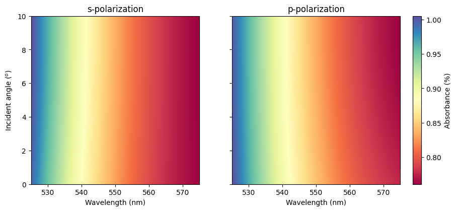
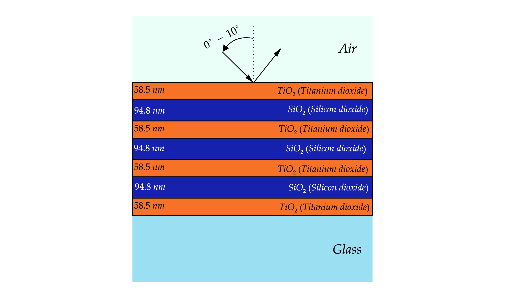
This notebook demonstrates how to calculate the reflectance of a multilayer thin-film stack designed as a 50:50 beam splitter deposited on a glass substrate. The reflectance is computed for both s-polarization and p-polarization across a wavelength range of 525 nm to 575 nm, and for incident angles from 0° to 10°.
Introduction
We will use the Transfer Matrix Method (TMM) to analyze the reflectance and transmittance of a multilayer thin-film structure designed to function as a 50:50 beam splitter in the visible spectrum. The multilayer consists of alternating layers of Titanium Dioxide (TiO₂) and Silicon Dioxide (SiO₂) deposited on a glass substrate, with air as the incident medium.
In this example, the calculation is done for two polarizations:
s-polarization: Electric field perpendicular to the plane of incidence.
p-polarization: Electric field parallel to the plane of incidence.
We will calculate the reflectance as a function of wavelength and angle of incidence for each polarization.
Materials and Layer Thickness
We are considering the following material stack:
Air as the incident medium.
TiO₂ (Titanium Dioxide) with a thickness of 58.5 nm.
SiO₂ (Silicon Dioxide) with a thickness of 94.8 nm.
SiO₂ (Silicon Dioxide) as the glass substrate.
[ ]:
# Define the materials and their thicknesses
material_list =  ["Air", "TiO2", "SiO2","TiO2","SiO2","TiO2","SiO2","TiO2", "SiO2"]
thickness_list = jnp.array([58.5e-9, 94.8e-9,58.5e-9, 94.8e-9,58.5e-9, 94.8e-9,58.5e-9])

# Define the wavelength range (525 nm to 575 nm) and angles of incidence (0° to 10°)
wavelength_arr = jnp.linspace(525e-9, 575e-9, 1000)
angle_of_incidences = jnp.linspace(0, (10*jnp.pi/180), 1000)

# Calculate reflectance for s-polarization
result_s = tmm(material_list=material_list, thickness_list=thickness_list,
             wavelength_arr=wavelength_arr, angle_of_incidences=angle_of_incidences,
             polarization="s")

# Calculate reflectance for p-polarization
result_p = tmm(material_list=material_list, thickness_list=thickness_list,
             wavelength_arr=wavelength_arr, angle_of_incidences=angle_of_incidences,
             polarization="p")
Reflectance Results
[ ]:
# Set up figure and image grid
fig = plt.figure(figsize=(10, 5))

grid = ImageGrid(fig, 111,
                 nrows_ncols=(1,2),
                 axes_pad=0.65,
                 share_all=True,
                 cbar_location="right",
                 cbar_mode="single",
                 cbar_size="5%",
                 cbar_pad=0.25,
                 )

# Add data to image grid
i = 0
for ax in grid:
    if i == 0:
        im = ax.imshow(result_s[1]*100, cmap='Spectral', aspect=50/10,extent = [525, 575, 0, 10])
        ax.set_title("s-polarization")
    if i ==1:
        im = ax.imshow(result_p[1]*100, cmap='Spectral', aspect=50/10,extent = [525, 575, 0, 10])
        ax.set_title("p-polarization")
    ax.set_xlabel("Wavelength (nm)")
    ax.set_ylabel("Incident angle ($^o$)")
    i += 1

# Colorbar
ax.cax.colorbar(im, label='Reflectance (%)')

plt.savefig("beam_splitter_reflectance_s_p.png", dpi=600)
plt.show()

Transmittance Results
[ ]:
# Set up figure and image grid
fig = plt.figure(figsize=(10, 5))

grid = ImageGrid(fig, 111,
                 nrows_ncols=(1,2),
                 axes_pad=0.65,
                 share_all=True,
                 cbar_location="right",
                 cbar_mode="single",
                 cbar_size="5%",
                 cbar_pad=0.25,
                 )

# Add data to image grid
i = 0
for ax in grid:
    if i == 0:
        im = ax.imshow(result_s[1]*100, cmap='Spectral', aspect=50/10,extent = [525, 575, 0, 10])
        ax.set_title("s-polarization")
    if i ==1:
        im = ax.imshow(result_p[1]*100, cmap='Spectral', aspect=50/10,extent = [525, 575, 0, 10])
        ax.set_title("p-polarization")
    ax.set_xlabel("Wavelength (nm)")
    ax.set_ylabel("Incident angle ($^o$)")
    i += 1

# Colorbar
ax.cax.colorbar(im, label='Transmittance (%)')

plt.savefig("beam_splitter_transmittance_s_p.png", dpi=600)
plt.show()

Absorbance Results
[ ]:
# Set up figure and image grid
fig = plt.figure(figsize=(10, 5))

grid = ImageGrid(fig, 111,
                 nrows_ncols=(1,2),
                 axes_pad=0.65,
                 share_all=True,
                 cbar_location="right",
                 cbar_mode="single",
                 cbar_size="5%",
                 cbar_pad=0.25,
                 )

# Add data to image grid
i = 0
for ax in grid:
    if i == 0:
        im = ax.imshow((1 -result_s[0] - result_s[1])*100, cmap='Spectral', aspect=50/10,extent = [525, 575, 0, 10])
        ax.set_title("s-polarization")
    if i ==1:
        im = ax.imshow((1 -result_p[0] - result_p[1])*100, cmap='Spectral', aspect=50/10,extent = [525, 575, 0, 10])
        ax.set_title("p-polarization")
    ax.set_xlabel("Wavelength (nm)")
    ax.set_ylabel("Incident angle ($^o$)")
    i += 1

# Colorbar
ax.cax.colorbar(im, label='Absorbance (%)')

plt.savefig("beam_splitter_absorbance_s_p.png", dpi=600)
plt.show()