Python Tutorial Notebook

1. Python Syntax

Text: Python Syntax Overview

Python is known for its clean and easy-to-read syntax. Unlike languages such as C or C++, Python does not use curly brackets ({}) to define blocks of code. Instead, it uses indentation to indicate a block of code. This makes Python code visually neat and eliminates the need for excessive symbols.

Python is an interpreted language, meaning the code is executed line by line, making it easy to debug and test. In contrast, C and C++ are compiled languagess, meaning the entire code is converted into machine code before execution. This often results in faster performance for C/C++ programs but makes debugging slightly more complex.

Example: Print Function

The print() function is used to output text in Python. This is simpler than the printf function in C or C++.

C Example:

#include <stdio.h>
int main() {
    printf("Hello, World!\n");
    return 0;
}

Python Equivalent:

print("Hello, World!")

# Example 1: Proper indentation
if True:
    print("This is correctly indented.")

This is correctly indented.

# Example 2: Incorrect indentation will throw an error
# Uncomment the following code to see the error
# if True:
# print("This will cause an IndentationError.")

# Example 3: Conditional statement
x = 10
y = 20
if x < y:
    print(f"{x} is less than {y}")

10 is less than 20

# Example 4: Loop with proper indentation
for i in range(5):
    print(f"Current number: {i}")

Current number: 0
Current number: 1
Current number: 2
Current number: 3
Current number: 4

# Example 5: Function definition and indentation
def greet(name):
    print(f"Hello, {name}!")
greet("Alice")

Hello, Alice!

# Example 6: Nested indentation
for i in range(3):
    if i % 2 == 0:
        print(f"{i} is even")

0 is even
2 is even

# Example 7: Multi-line statement
if (10 > 5 and
    20 > 15):
    print("Both conditions are True")

Both conditions are True

# Example 8: Inline comments
x = 10  # Assigning value to x
print(x)

10

# Example 9: Using pass
for i in range(3):
    if i == 1:
        pass  # Do nothing
    else:
        print(i)

0
2

# Example 10: Using else with loops
for i in range(3):
    print(i)
else:
    print("Loop completed!")

0
1
2
Loop completed!

2. Python Variables

Text: Introduction to Variables

In Python, variables are used to store data. Unlike C or C++, you don’t need to declare the type of the variable. Python automatically infers the type based on the assigned value.

Casting

To explicitly convert a variable to a specific type, you can use casting.

Case-Sensitive Strings

Variable names in Python are case-sensitive. For instance, Name and name would be treated as two different variables.

Lists in Python

Python lists are versatile and can store multiple items in a single variable. Lists allow duplicates, and their elements are indexed. Lists can store elements of different data types, but you can also choose to use lists with consistent data types for clarity.

# Example 1: Variable assignment and type inference
x = 5       # Integer
y = 3.14    # Float
z = "Hello" # String
print(type(x))
print(type(y))
print(type(z))

<class 'int'>
<class 'float'>
<class 'str'>

# Example 2: Casting
x = int(3.14)  # Cast float to int
print(x)
y = str(123)   # Cast int to string
print(y)
z = float("4.56")  # Cast string to float
print(z)

3
123
4.56

# Example 3: Case sensitivity
Name = "Alice"
name = "Bob"
print(Name)
print(name)

Alice
Bob

# Example 4: Lists
my_list = [1, 2, 3, 3, 4]
print("List elements:", my_list)
print("List length:", len(my_list))

List elements: [1, 2, 3, 3, 4]
List length: 5

# Example 5: Lists with mixed data types
mixed_list = ["Alice", 30, True]
print(mixed_list)

['Alice', 30, True]

# Example 6: List indexing
fruits = ["apple", "banana", "cherry"]
print("First fruit:", fruits[0])
print("Last fruit:", fruits[-1])

First fruit: apple
Last fruit: cherry

# Example 7: List slicing
numbers = [0, 1, 2, 3, 4, 5]
print("First three numbers:", numbers[:3])
print("Last two numbers:", numbers[-2:])

First three numbers: [0, 1, 2]
Last two numbers: [4, 5]

# Example 8: Modifying list elements
fruits[1] = "blueberry"
print("Modified fruits list:", fruits)

Modified fruits list: ['apple', 'blueberry', 'cherry']

# Example 9: Appending items to a list
numbers.append(6)
print("After appending:", numbers)

After appending: [0, 1, 2, 3, 4, 5, 6]

# Example 10: Inserting items into a list
numbers.insert(2, 99)
print("After inserting at index 2:", numbers)

After inserting at index 2: [0, 1, 99, 2, 3, 4, 5, 6]

# Example 11: Removing items from a list
numbers.remove(99)
print("After removing 99:", numbers)

After removing 99: [0, 1, 2, 3, 4, 5, 6]

# Example 12: Checking existence in a list
print("apple" in fruits)
print("grape" not in fruits)

True
True

3. Python Operations

Text: Mathematical Operations in Python

Python provides all basic mathematical operations, such as addition (+), subtraction (-), multiplication (*), division (/), and modulo (%).

Multiplying Lists

If you multiply a list by a number, Python creates a new list that repeats the original list. To perform elementwise operations on lists, you need a library like NumPy.

# Example 1: Basic mathematical operations
x = 10
y = 3
print("Addition:", x + y)
print("Subtraction:", x - y)
print("Multiplication:", x * y)
print("Division:", x / y)
print("Modulo:", x % y)

Addition: 13
Subtraction: 7
Multiplication: 30
Division: 3.3333333333333335
Modulo: 1

# Example 2: Exponentiation and floor division
print("Exponentiation:", x ** y)
print("Floor Division:", x // y)

Exponentiation: 1000
Floor Division: 3

# Example 3: List multiplication
my_list = [1, 2, 3]
print("List multiplied by 3:", my_list * 3)  # Repeats the list

List multiplied by 3: [1, 2, 3, 1, 2, 3, 1, 2, 3]

# Example 4: Elementwise multiplication (requires NumPy)
# Uncomment the following to see the error if NumPy is not used
# print("Elementwise multiplication:", [i * 3 for i in my_list])

# Example 5: Using the round function
c = 10 / 3
print("Rounded division result:", round(c, 2))

Rounded division result: 3.33

# Example 6: Increment and decrement
x += 1
print("Incremented x:", x)
x -= 1
print("Decremented x:", x)

Incremented x: 11
Decremented x: 10

# Example 7: Comparison operators
print("x is greater than y:", x > y)
print("x is equal to y:", x == y)

x is greater than y: True
x is equal to y: False

# Example 8: List comprehensions with operations
squared_numbers = [i**2 for i in range(5)]
print("Squared numbers:", squared_numbers)

Squared numbers: [0, 1, 4, 9, 16]

NumPy Tutorial

1. Introduction:

What is NumPy?

NumPy is a Python library used for working with arrays.

It also has functions for working in the domain of linear algebra, Fourier transform, and matrices.

NumPy was created in 2005 by Travis Oliphant. It is an open-source project, and you can use it freely.

NumPy stands for Numerical Python.

In Python, we have lists that serve the purpose of arrays, but they are slow to process.

NumPy aims to provide an array object that is up to 50x faster than traditional Python lists.

The array object in NumPy is called ndarray. It provides a lot of supporting functions that make working with ndarray very easy.

Arrays are very frequently used in data science, where speed and resources are very important.

Why is NumPy Faster Than Lists?

NumPy arrays are stored at one continuous place in memory, unlike lists, so processes can access and manipulate them very efficiently.

This behavior is called locality of reference in computer science.

This is the main reason why NumPy is faster than lists. Also, it is optimized to work with the latest CPU architectures.

Which Language is NumPy written in?

NumPy is a Python library and is written partially in Python, but most of the parts that require fast computation are written in C or C++.

Where is the NumPy Codebase?

The source code for NumPy is located at this GitHub repository: https://github.com/numpy/numpy

Array Creation in NumPy

Below are some examples of how to create arrays in NumPy:

import numpy as np

# Creating a 1D array
array_1d = np.array([1, 2, 3, 4, 5])
print("1D Array:", array_1d)

1D Array: [1 2 3 4 5]

# Creating a 2D array
array_2d = np.array([[1, 2, 3], [4, 5, 6]])
print("\n2D Array:")
print(array_2d)

2D Array:
[[1 2 3]
 [4 5 6]]

# Creating a 3D array
array_3d = np.array([[[1, 2], [3, 4]], [[5, 6], [7, 8]]])
print("\n3D Array:")
print(array_3d)

3D Array:
[[[1 2]
  [3 4]]

 [[5 6]
  [7 8]]]

# Creating an array with zeros
zeros_array = np.zeros((3, 3))
print("\nZeros Array:")
print(zeros_array)

Zeros Array:
[[0. 0. 0.]
 [0. 0. 0.]
 [0. 0. 0.]]

# Creating an array with ones
ones_array = np.ones((2, 4))
print("\nOnes Array:")
print(ones_array)

Ones Array:
[[1. 1. 1. 1.]
 [1. 1. 1. 1.]]

# Creating an array with a range of numbers
range_array = np.arange(1, 10, 2)  # start, stop, step
print("\nRange Array:", range_array)

Range Array: [1 3 5 7 9]

# Creating an array with evenly spaced numbers
linspace_array = np.linspace(0, 1, 5)  # start, stop, number of points
print("\nLinspace Array:", linspace_array)

Linspace Array: [0.   0.25 0.5  0.75 1.  ]

# Creating an identity matrix
identity_matrix = np.eye(3)
print("\nIdentity Matrix:")
print(identity_matrix)

Identity Matrix:
[[1. 0. 0.]
 [0. 1. 0.]
 [0. 0. 1.]]

2. Array Indexing and Array Slicing

Indexing in NumPy Arrays

# Accessing elements in a 1D array
print(array_1d[0])  # First element
print(array_1d[-1]) # Last element

1
5

# Accessing elements in a 2D array
print(array_2d[0, 1])  # Element in the first row and second column
print(array_2d[1, -1]) # Element in the last row and last column

2
6

Slicing NumPy Arrays

# Slicing a 1D array
print(array_1d[1:4])

[2 3 4]

# Slicing a 2D array
print(array_2d[0:2, 1:3])

[[2 3]
 [5 6]]

Array Shape and Iteration

# Shape of an array
print(array_2d.shape)

(2, 3)

# Iterating through an array
for row in array_2d:
    print(row)

[1 2 3]
[4 5 6]

# Flattening and iterating
for element in array_2d.flat:
    print(element)

1
2
3
4
5
6

Joining Arrays

# Joining arrays vertically
vstack_array = np.vstack((array_1d, array_1d))
print("\nVertical Stack:")
print(vstack_array)

Vertical Stack:
[[1 2 3 4 5]
 [1 2 3 4 5]]

# Joining arrays horizontally
hstack_array = np.hstack((array_1d, array_1d))
print("\nHorizontal Stack:")
print(hstack_array)

Horizontal Stack:
[1 2 3 4 5 1 2 3 4 5]

3. Random

Properties of Random in NumPy

# Generating random numbers
random_array = np.random.rand(3, 3)  # Uniform distribution between 0 and 1
print("\nRandom Array:")
print(random_array)

Random Array:
[[0.19613654 0.66699566 0.64752084]
 [0.41378751 0.77344783 0.09557272]
 [0.68367106 0.46480407 0.16145855]]

# Normal distribution
normal_array = np.random.normal(0, 1, 5)  # mean, standard deviation, size
print("\nNormal Distribution:", normal_array)

Normal Distribution: [-0.01018828  0.17432043  0.63089233 -0.35371924 -0.54080941]

# Binomial distribution
binomial_array = np.random.binomial(n=10, p=0.5, size=5)  # trials, probability, size
print("\nBinomial Distribution:", binomial_array)

Binomial Distribution: [4 4 5 3 5]

# Poisson distribution
poisson_array = np.random.poisson(lam=3, size=5)  # lambda, size
print("\nPoisson Distribution:", poisson_array)

Poisson Distribution: [4 2 1 2 2]

4. Daily Use Functions

Trigonometric Functions

angles = np.array([0, np.pi / 2, np.pi])

# Sine and cosine
sin_values = np.sin(angles)
cos_values = np.cos(angles)
print("\nSine Values:", sin_values)
print("Cosine Values:", cos_values)

# Tangent
tan_values = np.tan(angles)
print("\nTangent Values:", tan_values)

Sine Values: [0.0000000e+00 1.0000000e+00 1.2246468e-16]
Cosine Values: [ 1.000000e+00  6.123234e-17 -1.000000e+00]

Tangent Values: [ 0.00000000e+00  1.63312394e+16 -1.22464680e-16]

Other Useful Functions

# Square root
sqrt_array = np.sqrt(array_1d)
print("\nSquare Roots:", sqrt_array)

# Exponent
exp_array = np.exp(array_1d)
print("\nExponential:", exp_array)

# Logarithm
log_array = np.log(array_1d)
print("\nLogarithm:", log_array)

# Mean, Median, and Standard Deviation
mean_value = np.mean(array_1d)
median_value = np.median(array_1d)
std_value = np.std(array_1d)
print("\nMean:", mean_value)
print("Median:", median_value)
print("Standard Deviation:", std_value)

Square Roots: [1.         1.41421356 1.73205081 2.         2.23606798]

Exponential: [  2.71828183   7.3890561   20.08553692  54.59815003 148.4131591 ]

Logarithm: [0.         0.69314718 1.09861229 1.38629436 1.60943791]

Mean: 3.0
Median: 3.0
Standard Deviation: 1.4142135623730951

Matplotlib Python Tutorial

Introduction:

What is Matplotlib?

Matplotlib is a low-level graph plotting library in Python that serves as a visualization utility.

• Matplotlib was created by John D. Hunter.

• Matplotlib is open source, and we can use it freely.

• It is mostly written in Python, with a few segments written in C, Objective-C, and JavaScript for platform compatibility.

Where is the Matplotlib Codebase?

The source code for Matplotlib is located at this GitHub repository: Matplotlib GitHub Repository

---

Pyplot

The pyplot module in Matplotlib provides a state-based interface to Matplotlib. It contains functions that are closely aligned with MATLAB-style plotting commands.

### Plot Example 1: Simple Line Plot

import matplotlib.pyplot as plt

# Simple Line Plot
x = [0, 1, 2, 3, 4, 5]
y = [0, 1, 4, 9, 16, 25]

plt.plot(x, y, label='y = x^2', color='blue', marker='o')
plt.title('Simple Line Plot')
plt.xlabel('X-Axis')
plt.ylabel('Y-Axis')
plt.legend()
plt.grid(True)
plt.show()

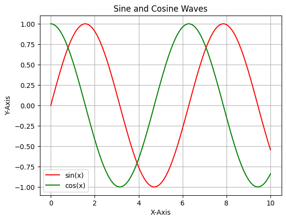
### Plot Example 2: Multiple Lines in One Plot

import numpy as np

# Data for multiple lines
x = np.linspace(0, 10, 100)
y1 = np.sin(x)
y2 = np.cos(x)

plt.plot(x, y1, label='sin(x)', color='red')
plt.plot(x, y2, label='cos(x)', color='green')
plt.title('Sine and Cosine Waves')
plt.xlabel('X-Axis')
plt.ylabel('Y-Axis')
plt.legend()
plt.grid(True)
plt.show()

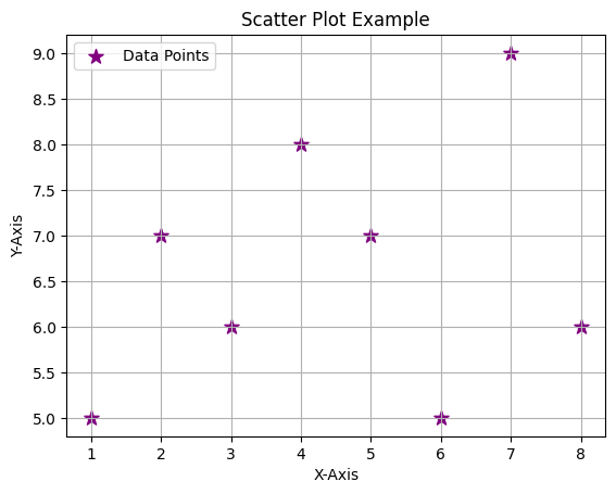
### Plot Example 3: Scatter Plot

# Scatter Plot
x = [1, 2, 3, 4, 5, 6, 7, 8]
y = [5, 7, 6, 8, 7, 5, 9, 6]

plt.scatter(x, y, label='Data Points', color='purple', marker='*', s=100)
plt.title('Scatter Plot Example')
plt.xlabel('X-Axis')
plt.ylabel('Y-Axis')
plt.legend()
plt.grid(True)
plt.show()

### Imshow Example 1: Visualizing a 2D Array

# Imshow with Random Data
import numpy as np

# Generating random data
random_data = np.random.rand(10, 10)

plt.imshow(random_data, cmap='viridis', interpolation='nearest')
plt.colorbar(label='Random Values')
plt.title('Imshow Example: Random Data')
plt.show()

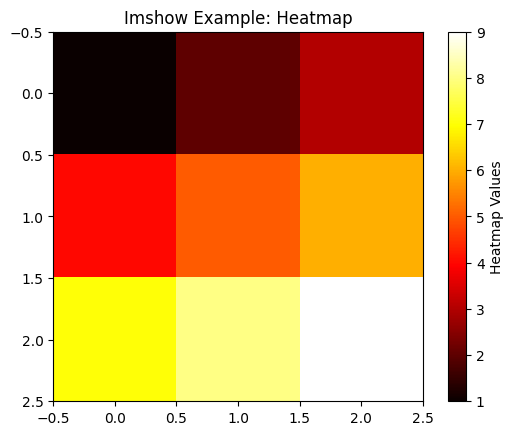
### Imshow Example 2: Heatmap Representation


# Imshow with Heatmap
heatmap_data = np.array([[1, 2, 3], [4, 5, 6], [7, 8, 9]])

plt.imshow(heatmap_data, cmap='hot', interpolation='nearest')
plt.colorbar(label='Heatmap Values')
plt.title('Imshow Example: Heatmap')
plt.show()